project airfoil: Potential Flow Visualization

Introduction

Fluid dynamics, for all its mathematical complexity, is unique in that it allows for the visualization of a myriad of interesting topics that can help one better understand the underlying theory and its practical effects. To that end, I decided to dip my toes into this subject and created a simple 2D potential flow visualizer in OpenGL/C++, but before we get into the code details I'll provide an extremely brief overview of this subject below.

Potential Flow Theory Basics

Potential flow theory seeks to describe irrotational velocity fields through their corresponding velocity gradient, often called the velocity's potential:

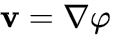
And corresponding stream function (for 2D cases only):

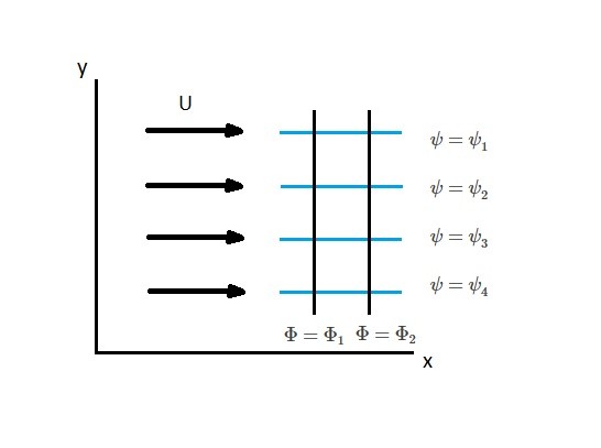
While the math isn't too convoluted, it's not entirely trivial to see how exactly these functions model velocity field behavior. Images like this one alleviate this question quite handily:

In the above case we have a flow entering a pipe in the top-left corner, and exiting in the bottom-right. Each green and red line depicts a direction along which the stream and potential functions, respectively, are constant. From this it becomes clear that the stream function models the path particles will take when suspended in and carried by the fluid, while the potential function is an analogous term whose lines of constant potential run perpendicular to the streamlines.

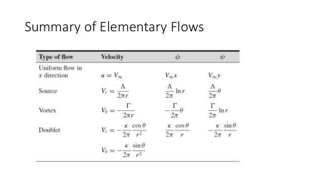
While typically used for noncompressible simulation, such as approximating water's behavior, the theory can be applied to compressible flows as well, like in the case of modeling the outer flow of various airfoils. Such flows are generally quite complex, but there are simple cases - known as "elementary flows" - that can be solved analytically and superimposed on one another to accurately approximate the desired situation. In particular, the four most commonly-utilized elementary flows include:

Uniform Flow -
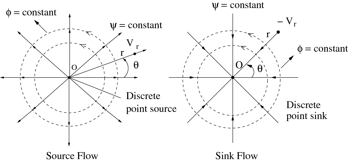
Source/Sink Flow-
Vortex Flow-
Doublet Flow-

And whose mathematical descriptions are summarized in the following table:

So, for the following project I decided to visualize the velocity, potential, and stream fields of such user-created superpositions, as can be seen in the following demo:

Let's get into some of the particulars behind this little program:

In Practice

Flow Definition

In order to model any potential flows, one first needs to define what a flow is in the given context. In this case, I decided to define a struct called flow that houses its most essential properties - the velocity, stream, and potential values as calculated from the above table:

struct Flow
{
 std::vector<float> velocity;
 std::vector<float> potential;
 std::vector<float> stream;
};

The four aforementioned flows are then defined, alongside some other important parameters and functions, in the class Field:

class Field
{
public:
 bool updateField, updateWindow, uniformBool = false, sourceBool = true, vortexBool = false, doubletBool = false, showOrigin = true, pointSelected = false, change, del = false;
 int showBackground = 0, pixelSize = 1, ID;
 std::vector<float> velocityPoints, velocityColors, origin, originColors, stream, streamColors, potential, potentialColors, background, flowType;
 float minStream = 10000.0f, maxStream = -10000.0f, minPotential = 10000.0f, maxPotential = -10000.0f, minVel = 10000.0f, maxVel = -10000.0f;

 void Clear();
 void InitializeField();
 void ReinitializeField(std::vector<float> &points);
 void UpdateField(std::vector<float> &points);
 Flow Uniform(std::vector<float> &points, float xDisplacement, float yDisplacement, float speed, float flowAngle);
 Flow Source(std::vector<float> &points, float xDisplacement, float yDisplacement, float flowRate);
 Flow Vortex(std::vector<float> &points, float xDisplacement, float yDisplacement, float circulation);
 Flow Doublet(std::vector<float> &points, float xDisplacement, float yDisplacement, float strength);
 void InitializeNewFlow(Flow &flow, std::vector<float> &points);
 void UpdateSelectedFlow(int ID, Flow &flow, std::vector<float> &points, bool del);
};

Note that for every member of Flow there are some corresponding vectors in Field - Flow::velocity matches with Field::velocityPoints and Field::velocityColors, Flow::potential with Field::potentialColors, and so on. These latter vectors end up storing the superimposed member values and/or colors as the user continues adding, adjusting, and deleting elementary flows from the window. In addition, we have the int pixelSize which sets the screen resolution, and vector flowType that holds a flow's ID, origin position, and strength.

Initialization

Now that we've defined our four-flow library, we need to populate each one with the relevant velocity, potential, and stream data as dictated by their origin position and defining formulas (which have been converted to Cartesian coordinates for simplicity's sake). As an example, here is the code for the source flow:

Flow Field::Source(std::vector<float> &points, float xDis, float yDis, float Q)
{
 float x, y;
 for (int i = 0; i < (int)(0.25f * points.size()); ++i)
 {
  x = __velocityContainer[4 * i + 2] - xDis; y = __velocityContainer[4 * i + 3] - yDis;

  source.velocity[2 * i] = (Q / (2 * 3.1415926f)) * (x / (x * x + y * y));
  source.velocity[2 * i + 1] = (Q / (2 * 3.1415926f)) * (y / (x * x + y * y));
 }

 int __count = -1;
 for (int j = 0; j < glutGet(GLUT_WINDOW_HEIGHT); j += pixelSize)
 {
  for (int i = 0; i < glutGet(GLUT_WINDOW_WIDTH); i += pixelSize)
  {
   ++__count;
   source.stream[__count] = (Q / (2 * 3.1415926f)) * abs(atan((j - yDis) / (i - xDis)));
   if ((i - xDis) * (i - xDis) + (j - yDis) * (j - yDis) != 0) 
    source.potential[__count] = (Q / (2 * 3.1415926f)) * log(sqrt(abs((i - xDis) * (i - xDis) + (j - yDis) * (j - yDis))));
  }
 }

 return source;
}

The stream and potential functions are easy enough to understand - simply use the given equations to calculate those parameters' values at every point on the screen, relative to its point of origin. The velocity, however, is a little trickier. Because the velocity field is made up of vector rather than scalar values, we need to draw a series of oriented lines to represent this fact, as can be seen in the demo video. These lines are then evenly spread amongst one another so as to not cover up the entire screen, hence why we don't iterate across the entire window's pixel dimensions when dealing with them. How exactly these line positions/orientations are determined, though, requires a broader discussion of the code's basic update structure.

To better describe what's going on, we first need to introduce a few other local variables that need to be initialized upon runtime before anything can be simulated on-screen:

std::vector<float> __velocity, __tempVelocity, __velocityContainer,

__velocityMagnitude, __tempStream, __streamContainer, __tempPotential,

__potentialContainer;

The superposition of different elementary flows, and subsequent vector field definition, is only made possible thanks to the inputted data these vectors store. Here's how it works:

Velocity:

Clear out all vectors, variables, etc., and create all of the lines that will represent the velocity field:

void Field::InitializeField()
{
 this->Clear();
 //velocity lines
 for (float y = 0; y <= glutGet(GLUT_WINDOW_HEIGHT); y += 20)
 {
  for (float x = 0; x <= glutGet(GLUT_WINDOW_WIDTH); x += 20)
  {
   velocityPoints.push_back(x);
   velocityPoints.push_back(y);
   velocityPoints.push_back(x + 10);
   velocityPoints.push_back(y);
  }
 }
}

void Field::InitializeField()
{
 ...
 //velocity lines and associated colors
 for (int i = 0; i < (int)(0.5f * velocityPoints.size()); ++i)
 {
  velocityColors.push_back(1);
  velocityColors.push_back(1);
  velocityColors.push_back(1);

  __velocity.push_back(0);
  __velocityMagnitude.push_back(0);

  uniform.velocity.push_back(0);
  source.velocity.push_back(0);
  vortex.velocity.push_back(0);
  doublet.velocity.push_back(0);
 }

 for (auto i : velocityPoints) __tempVelocity.push_back(i);
 ...
}

Initialize the flow in the so-called InitializeNewFlow method. This function, and its corresponding update sister, comprise the heart of this little project since they combine all flows instantiated by the user together to calculate/visualize the resulting flow conditions. First up, every time a new flow is initialized, we push back that flow's velocity data into the local variable __velocityContainer:

void Field::InitializeNewFlow(Flow &flow, std::vector<float> &points)
{
 ...
 for (int i = 0; i < (int)(0.5f * points.size()); ++i) __velocityContainer.push_back(flow.velocity[i]);
 ...
}

Then, iterating across the entirety of our __velocity vector, which will contain the updated, superimposed velocity data, we loop through each individual flow stored in __velocityContainer and increment the corresponding __velocity value by that amount, essentially combining the separate velocity fields into one:

void Field::InitializeNewFlow(Flow &flow, std::vector<float> &points)
{
 ...
 for (int i = 0; i < (int)(0.25f * points.size()); ++i)
 {
  __velocity[2 * i] = __velocity[2 * i + 1] = 0;
  for (int j = 0; j < (int)__velocityContainer.size(); j += (int)(0.5f * points.size()))
  {
   __velocity[2 * i] += __velocityContainer[2 * i + j];
   __velocity[2 * i + 1] += __velocityContainer[2 * i + 1 + j];
  }
 }
 ...
}

Finally, after constricting the velocity magnitudes to some predetermined maximum value (to ensure that the rendered lines aren't ridiculously long), we set the correct vector size/direction by adding the calculated velocity at a given position to the hard-set point from which that line originates:

void Field::InitializeNewFlow(Flow &flow, std::vector<float> &points)
{
 ...
 for (int i = 0; i < (int)(0.25f * points.size()); ++i)
 {
  points[4 * i + 2] = __tempVelocity[4 * i] + __velocity[2 * i];
  points[4 * i + 3] = __tempVelocity[4 * i + 1] + __velocity[2 * i + 1];
  __tempVelocity[4 * i + 2] = points[4 * i + 2];
  __tempVelocity[4 * i + 3] = points[4 * i + 3];
 }
 ...
}

Stream/Potential:

The process used to initialize the stream/potential fields is very similar to the one described above for the velocity, and applies to both of the former cases. The one key difference is that these fields store relevant data for the entirety of the working environment rather than just a series of lines representing vectors in 2D space, and thus need to be iterated over all rasterized on-screen pixels. To reflect this difference, all we need to do is change the initialization loop that correctly sets the parameter sizes:

void Field::InitializeField()
{
 ...
 for (int j = 0; j < glutGet(GLUT_WINDOW_HEIGHT); j += pixelSize)
 {
  for (int i = 0; i < glutGet(GLUT_WINDOW_WIDTH); i += pixelSize)
  {
   //background colors
   background.push_back(i);
   background.push_back(j);

   //streamlines
   uniform.stream.push_back(0);
   source.stream.push_back(0);
   vortex.stream.push_back(0);
   doublet.stream.push_back(0);

   __tempStream.push_back(0);

   streamColors.push_back(0);
   streamColors.push_back(0);
   streamColors.push_back(0);

   //potential lines
   uniform.potential.push_back(0);
   source.potential.push_back(0);
   vortex.potential.push_back(0);
   doublet.potential.push_back(0);

   __tempPotential.push_back(0);

   potentialColors.push_back(0);
   potentialColors.push_back(0);
   potentialColors.push_back(0);
  }
 }
 ...
}

Before setting the respective field containers and combining each new field's values to form the superimposed solution, just like the velocity:

void Field::InitializeNewFlow(Flow &flow, std::vector<float> &points)
{
 ...
 for (int i = 0; i < (int)flow.stream.size(); ++i)
  __streamContainer.push_back(flow.stream[i]);

 for (int i = 0; i < (int)__tempStream.size(); ++i) __tempStream[i] = 0;

 for (int j = 0; j < (int)__streamContainer.size(); j += flow.stream.size())
  for (int i = 0; i < (int)flow.stream.size(); ++i)
   __tempStream[i] += __streamContainer[i + j];
 for (int i = 0; i < (int)flow.potential.size(); ++i)
  __potentialContainer.push_back(flow.potential[i]);

 for (int i = 0; i < (int)__tempPotential.size(); ++i) __tempPotential[i] = 0;

 for (int j = 0; j < (int)__potentialContainer.size(); j += flow.potential.size())
  for (int i = 0; i < (int)flow.potential.size(); ++i)
   __tempPotential[i] += __potentialContainer[i + j];
 ...
}

Visually Representing the Data

With our flow data initialized, we now need to somehow draw the results on-screen. The velocity field lines are already in place at this point, but we still need to somehow color them and the stream/potential functions to signal their respective magnitudes. This is accomplished with the following gradient generation function, which creates a color ramp for a given set of data by subdividing the minimum and maximum values into four equal parts, assigning those ranges different RGB color spectrums, and storing the results in a vector:

void Utility::SetGradient(std::vector<float> &colors, std::vector<float> &values, float &min, float &step)
{
 for (int i = 0; i < (int)(values.size()); ++i)
 {
  if (values[i] < min + step)
  {
   colors[3 * i] = 0;
   colors[3 * i + 1] = 0;
   colors[3 * i + 2] = (values[i] - min) / step;
  }

  else if (values[i] < min + 2 * step)
  {
   colors[3 * i] = 0;
   colors[3 * i + 1] = (values[i] - (min + step)) / step;
   colors[3 * i + 2] = 1 - (values[i] - (min + step)) / step;
  }

  else if (values[i] < min + 3 * step)

  {
   colors[3 * i] = (values[i] - (min + 2 * step)) / step;
   colors[3 * i + 1] = 1;
   colors[3 * i + 2] = 0;
  }

  else
  {
   colors[3 * i] = 1;
   colors[3 * i + 1] = 1 - (values[i] - (min + 3 * step)) / step;
   colors[3 * i + 2] = 0;
  }
 }
}

For this specific program I decided to set the bottom 25% equal to colors between black and blue, the 25-50% equal to colors between blue and green, 50-75% to green and yellow, and 75-100% to yellow and red. We can then invoke this function for each flow attribute and switch between the resultant color vectors while rendering whenever we would like to see a specific result:

utility.SetGradient(velocityColors, __velocityMagnitude, minVel, __velStep);
utility.SetGradient(streamColors, __tempStream, minStream, __streamStep);
utility.SetGradient(potentialColors, __tempPotential, minPotential, __potentialStep);

Note that each __step float is just the (max - min) / 4 of that specific trait, and that for the velocity field we are coloring each line based on its magnitude, which we calculate like so:

for (int i = 0; i < (int)(0.25f * points.size()); ++i)
 __velocityMagnitude[2 * i] = __velocityMagnitude[2 * i + 1] = sqrt(__velocity[2 * i] * __velocity[2 * i] + __velocity[2 * i + 1] * __velocity[2 * i + 1]);

Updating the Field

Now that field initialization can be done successfully, we need to establish some methods to allow for user interactivity with the program, namely adding, moving, and deleting flows, all of which are handled by a separate Utility class. Let's address these one-by-one.

Adding Flows

The simplest case is adding a flow, in which case we simply need to call the initialization method that takes care of all the functionality described thus far. For example, if we wish to add a source flow, then the code looks like this:

void Utility::AddFlow()
{
 if (input.rightMouseButtonPressed)
 {
  field.origin.push_back(input.initialRightMousePosition.x);
  field.origin.push_back(input.initialRightMousePosition.y);

  ...
  else if (field.sourceBool)
  {
   field.originColors.push_back(1);
   field.originColors.push_back(0);
   field.originColors.push_back(0);

   field.flowType.push_back(1);
   field.flowType.push_back(input.initialRightMousePosition.x);
   field.flowType.push_back(input.initialRightMousePosition.y);
   field.flowType.push_back(2500);

   source = field.Source(field.velocityPoints, input.initialRightMousePosition.x, input.initialRightMousePosition.y, 2500);
   field.InitializeNewFlow(source, field.velocityPoints);
   }
  ...

}
}

In addition to calling InitializeNewFlow, we also store the flow's point of origin, origin color (to aid with flow selection), type (uniform, source, vortex, or doublet), and strength for later use.

Selecting and Moving Flows

Next we look at how a flow is selected and dragged around using the mouse. To do this we first need to determine whether a flow has been clicked on (roughly around the origin) and, if so, what that flow's ID (determined from the order in which flows have been added/deleted) is:

void Utility::SelectFlow()
{
 if (input.leftMouseButtonPressed)
 {
  field.pointSelected = false;
  for (int i = 0; i < (int)(0.5f * field.origin.size()); ++i)
  {
   if (input.initialLeftMousePosition.x >= field.origin[2 * i] - 15.0f && input.initialLeftMousePosition.x <= field.origin[2 * i] + 15.0f && input.initialLeftMousePosition.y >= field.origin[2 * i + 1] - 15.0f && input.initialLeftMousePosition.y <= field.origin[2 * i + 1] + 15.0f)
   {
    __xPos = 2 * i; //selected simple flow origin point (x-value)
    __yPos = 2 * i + 1; //selected simple flow origin point (y-value)
    field.ID = i; //selected simple flow ID
    field.pointSelected = true;
   }
  }

  input.leftMouseButtonPressed = false;
  field.updateField = true;
 }
}

More specifically, a flow's ID is found based on its origin's index in the corresponding storage vector. Then, we simply determine the flow's type based on its ID, call the UpdateSelectedField function, and reset the selected flow (with the correct type - in this example the source flow) by setting origin to equal the mouse's current position:

void Utility::MoveFlow()
{
 if (input.leftMouseButtonDown)
 {
  if (field.pointSelected)
  {
   field.origin[__xPos] = input.leftMousePosition.x;
   field.origin[__yPos] = input.leftMousePosition.y;
                
   ...
   if (field.flowType[4 * field.ID] == 1)
   {
    source = field.Source(field.velocityPoints, input.leftMousePosition.x, input.leftMousePosition.y, field.flowType[4 * field.ID + 3]);
    field.UpdateSelectedFlow(field.ID, source, field.velocityPoints, false);
   }

...

  }
 }
}

Conveniently-enough, UpdateSelectedFlow doesn't require too much explanation because it works in almost the exact same way as InitializeFlow! The only difference is that instead of pushing back and expanding the container storage vectors to accommodate new flows, we loop through them to find the selected flow's initial data entries, replace them with that flow's new values (based on the translation it undergoes that update cycle), and then use those numbers to calculate the flow conditions as described previously:

void Field::UpdateSelectedFlow(int c, Flow &flow, std::vector<float> &points, bool del)
{
 for (int i = (int)(c * 0.5f * points.size()); i < (int)((c + 1) * 0.5f * points.size()); ++i)
  __velocityContainer[i] = flow.velocity[i - (int)(c * 0.5f * points.size())];

 for (int i = (int)(c * flow.stream.size()); i < (int)((c + 1) * flow.stream.size()); ++i)
  __streamContainer[i] = flow.stream[i - (int)(c * flow.stream.size())];

 for (int i = (int)(c * flow.potential.size()); i < (int)((c + 1) * flow.potential.size()); ++i)
 __potentialContainer[i] = flow.potential[i - (int)(c * flow.potential.size())];

...

Deleting Flows

Lastly, flow deletion is handled by the following function, in which we erase the selected flow's origin and flow type information before reinitializing the entire field, this time without the deleted flow's influence:

void Utility::DeleteFlow()
{
 if (field.del)
 {
  field.updateField = true;

  field.origin.erase(field.origin.begin() + 2 * field.ID);
  field.origin.erase(field.origin.begin() + 2 * field.ID);

  field.originColors.erase(field.originColors.begin() + 3 * field.ID);
  field.originColors.erase(field.originColors.begin() + 3 * field.ID);
  field.originColors.erase(field.originColors.begin() + 3 * field.ID);

  field.flowType.erase(field.flowType.begin() + 4 * field.ID);
  field.flowType.erase(field.flowType.begin() + 4 * field.ID);
  field.flowType.erase(field.flowType.begin() + 4 * field.ID);
  field.flowType.erase(field.flowType.begin() + 4 * field.ID);

  field.InitializeField();
  field.ReinitializeField(field.velocityPoints);
 }
}

The reinitialization method called at the end behaves similarly to the Utility::Add function, except for one key difference: no new data is appended to the flowType vector, which means that the current flows (which were cleared out by field.InitializeField), other than the one just deleted, are being redrawn on-screen.

Final Details and Source Code

A few minor points I would like to bring up before wrapping this post up:

Resizing the window allows one to create more, or less, space in which flows can be applied and manipulated.
A key to the top-right shows the maximum and minimum magnitudes for the velocity, stream, or potential (depending on which mode one is in).
As of right now there is no way to change the flow strengths without diving into the source code itself. I might add this sort of UI functionality at a later time.
From time to time there are some rendering glitches that occur - mostly random pixels going dark and/or jumping around. You have been warned.
To draw the text, I used a custom-made character rendering library discussed in a previous post. It has been linked here for those interested in checking it out.

Finally, here is the build and source code for this project:

potential_flow_simulator

The hotkeys are:

Right-mouse click to add a new flow.
Left-mouse click to select and move flows. Do this by clicking on their colored origin points.
u - set uniform flow for drawing.
s - set source flow for drawing.
v - set vortex flow for drawing.
d - set doublet flow for drawing
Space bar - switch between displaying the velocity, stream, and potential fields on-screen.
del - delete the selected flow.
c - clear screen.
o - hide origin points.
up arrow - increase window resolution.
down arrow - decrease window resolution.

project airfoil

Pages

Friday, January 24, 2020

Potential Flow Visualization